2D datasets

This tutorial reproduces the two 2D datasets of the paper. In both, the source and target points are unpaired samples of two classes, and optimal transport with the squared Euclidean cost sends points to the wrong class. CloneOT learns the cost from correspondences between subsets of source and target points, which play the role of clones.

• T-shape shows that the cost must be learned. A vertical bar on the left moves to the right and a horizontal bar on top moves down, but moving the left bar down and the top bar to the right is cheaper under the squared Euclidean cost. The points form subsets of two source and two target points at one position of a bar, and the correspondences of 20% of the subsets are given.

• Rotated moons compares CloneOT with OT-SI, a discrete inverse OT solver that learns costs from subset correspondence. The target is the two moons rotated by 90 degrees, and the only correspondence is between each source moon and its rotated moon.

import numpy as np
import matplotlib.pyplot as plt
import cloneot as cot
from cloneot.datasets import class_accuracy, label_fraction, rotated_moons, t_shape

T-shape

We draw 400 training points, 400 new source points for testing, and a large reference sample of target points that tells which class a prediction lands on.

data, test, reference = t_shape(400, seed=0), t_shape(400, seed=100), t_shape(4000, seed=200)
labels = label_fraction(data['source_clone'], data['target_clone'], fraction=0.2, seed=0)
print(f"{len(data['source'])} source and {len(data['target'])} target points, "
      f"{len(set(labels[0]) - {-1})} corresponding subsets given")

400 source and 400 target points, 40 corresponding subsets given

Without correspondences, CloneOT is entropic optimal transport with the squared Euclidean cost, the solver underlying CellOT. With the correspondences, it learns the cost.

euclidean = cot.CloneOT().fit(data['source'], data['target']).fit_map()
cloneot = cot.CloneOT().fit(data['source'], data['target'], *labels).fit_map()

def summarize(model, test, reference):
    prediction = model.transport(test['source'])
    nearest = ((prediction[:, None] - reference['target'][None]) ** 2).sum(-1).argmin(1)
    correct = reference['target_class'][nearest] == test['source_class']
    error = np.linalg.norm(prediction - test['fate'](test['source']), axis=1).mean()
    return prediction, correct, error

fig, axes = plt.subplots(1, 2, figsize=(10, 3.8))
for ax, (name, model) in zip(axes, [('Squared Euclidean cost', euclidean), ('CloneOT', cloneot)]):
    prediction, correct, error = summarize(model, test, reference)
    cot.pl.transport(test['source'], test['target'], prediction, correct, ax=ax, legend=False,
                     title=f'{name}\n{correct.mean():.0%} on the correct bar, distance to fate {error:.2f}')
    ax.title.set_fontsize(10)
plt.tight_layout()

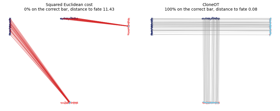
Red rays end on the wrong bar. The squared Euclidean cost sends the left bar down and the top bar to the right, whereas CloneOT places every new point on its own bar and recovers the translation of each bar.

Rotated moons

data, test, reference = rotated_moons(400, seed=0), rotated_moons(400, seed=100), rotated_moons(4000, seed=200)
labels = (data['source_clone'], data['target_clone'])        # the two moons are the corresponding subsets
euclidean = cot.CloneOT().fit(data['source'], data['target']).fit_map()
cloneot = cot.CloneOT().fit(data['source'], data['target'], *labels).fit_map()

fig, axes = plt.subplots(1, 2, figsize=(10, 4.4))
for ax, (name, model) in zip(axes, [('Squared Euclidean cost', euclidean), ('CloneOT', cloneot)]):
    prediction, correct, error = summarize(model, test, reference)
    cot.pl.transport(test['source'], test['target'], prediction, correct, ax=ax, legend=False,
                     title=f'{name}\n{correct.mean():.0%} on the correct moon, distance to fate {error:.2f}')
    ax.title.set_fontsize(10)
plt.tight_layout()

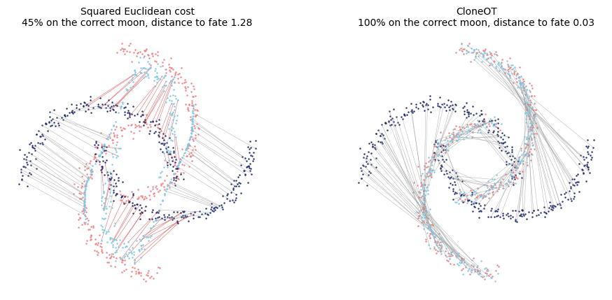
The only supervision is which moon corresponds to which rotated moon, without any pairs of points. CloneOT learns a cost under which the cheapest transport is the rotation itself.